WrensBookshelf

WrensBookshelf is a package for the R programming language that contains a collection of color palettes that were extracted from various books on my son's bookshelf. Also included are a number of functions and wrappers to utilize them in base R and ggplot2 plotting functions, as well as to subset the packages to desired number/specific colors. It was heavily inspired by and modeled after the MetBrewer, PNWColors, and wesanderson packages, and of course RColorBrewer, so if you are here you should check them out too! Logo designed using hexSticker and illustrator.

Installation

You can install the official released version of WrensBookshelf from CRAN using:

install.packages("WrensBookshelf")

And the developement version from Github using:

devtools::install_github("buveges/WrensBookshelf")

Palettes

All palettes

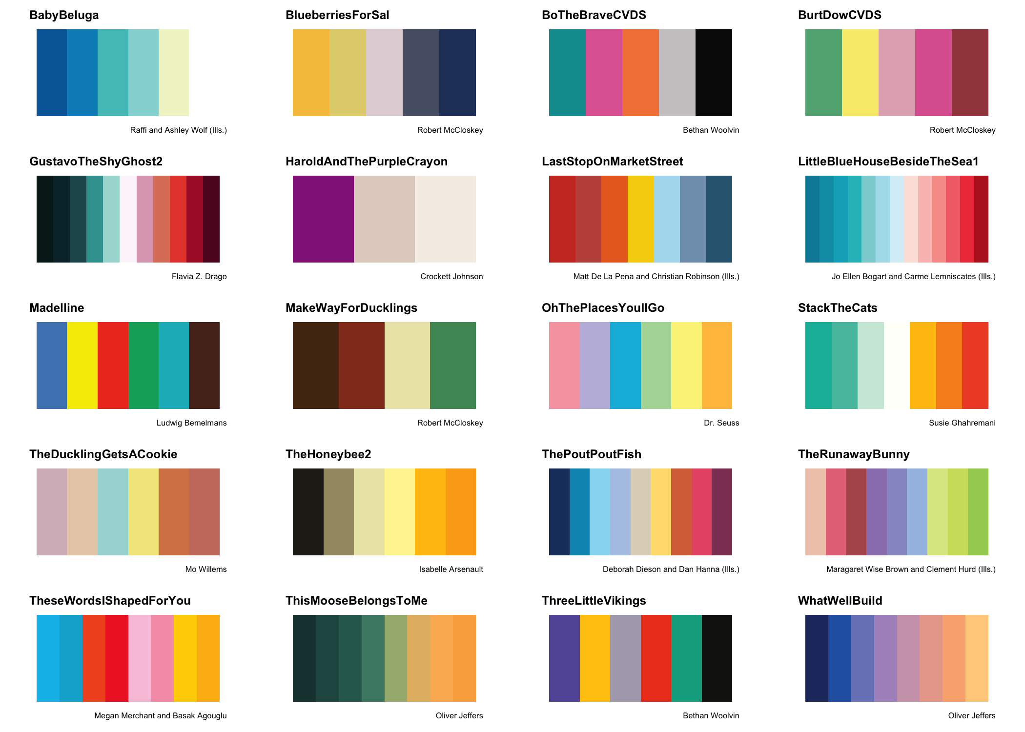
Can view all palettes from Wren’s bookshelf using the ShowBookshelf() function

library(WrensBookshelf)
ShowBookshelf()

names(WrensBookshelf)
#>  [1] "BabyBeluga"                   "BabyWrenAndTheGreatGift"     
#>  [3] "BatheTheCat"                  "BlueberriesForSal"           
#>  [5] "BoTheBrave"                   "BoTheBraveCVDS"              
#>  [7] "BurtDow"                      "BurtDowCVDS"                 
#>  [9] "CapsForSale"                  "GustavoTheShyGhost1"         
#> [11] "GustavoTheShyGhost2"          "HaroldAndThePurpleCrayon"    
#> [13] "JeffGoesWild"                 "JulienIsAMermaid"            
#> [15] "LastStopOnMarketStreet"       "LittleBlueHouseBesideTheSea1"
#> [17] "LittleBlueHouseBesideTheSea2" "Madelline"                   
#> [19] "MakeWayForDucklings"          "Moongame"                    
#> [21] "MoreThanALittle"              "OhThePlacesYoullGo"          
#> [23] "Opposites"                    "StackTheCats"                
#> [25] "TheDucklingGetsACookie"       "TheHoneybee1"                
#> [27] "TheHoneybee2"                 "ThePoutPoutFish"             
#> [29] "TheRunawayBunny"              "TheSnowyDay"                 
#> [31] "TheStoryOfBabar"              "TheseWordsIShapedForYou"     
#> [33] "ThisMooseBelongsToMe"         "ThreeLittleVikings"          
#> [35] "TigerDays"                    "TinyPerfectThings"           
#> [37] "Vampenguin"                   "WhatWellBuild"               
#> [39] "WhereTheWildThingsAre"        "YouMatter"

Color Vision Deficiency (CVD) safe palettes

Can display only CVD safe palettes using CVDsafe option. These were determined/assigned by using the amazing cvdPlot() function from the colorBlindness package, and should be safe for deuteranopia and protanopia, and in many cases when desaturated (BW).

ShowBookshelf(CVDsafe = TRUE)

Palettes for Discrete/Continuous data

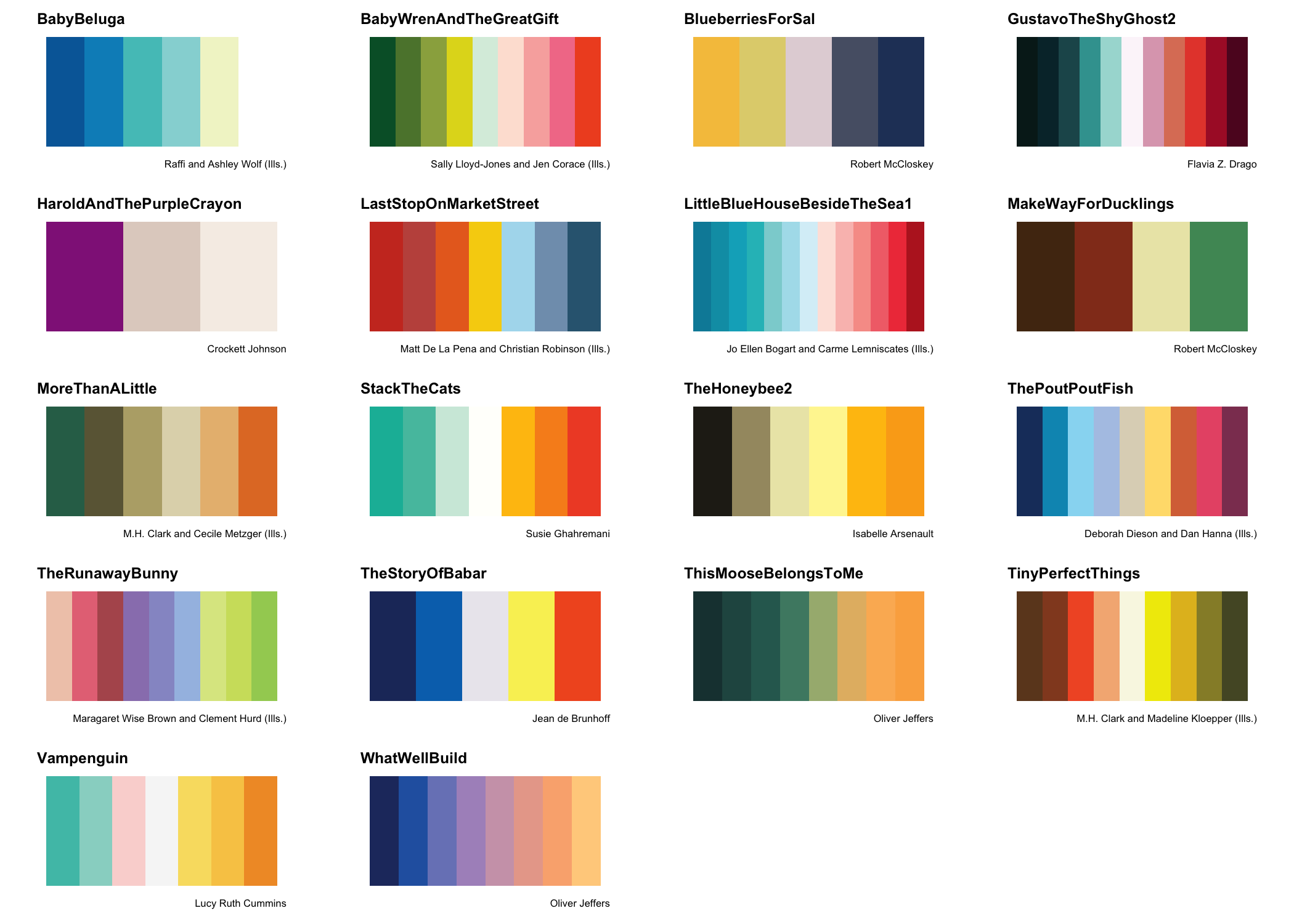
All palettes can be used for either discrete or continuous data display, however some apply themselves to one better than the other. Use the BestFor option to view palettes that, in my own view, work best for “discrete” or “continuous” variables. This can be combined/stacked with the CVDsafe option as well

ShowBookshelf(BestFor = "continuous")

Functions

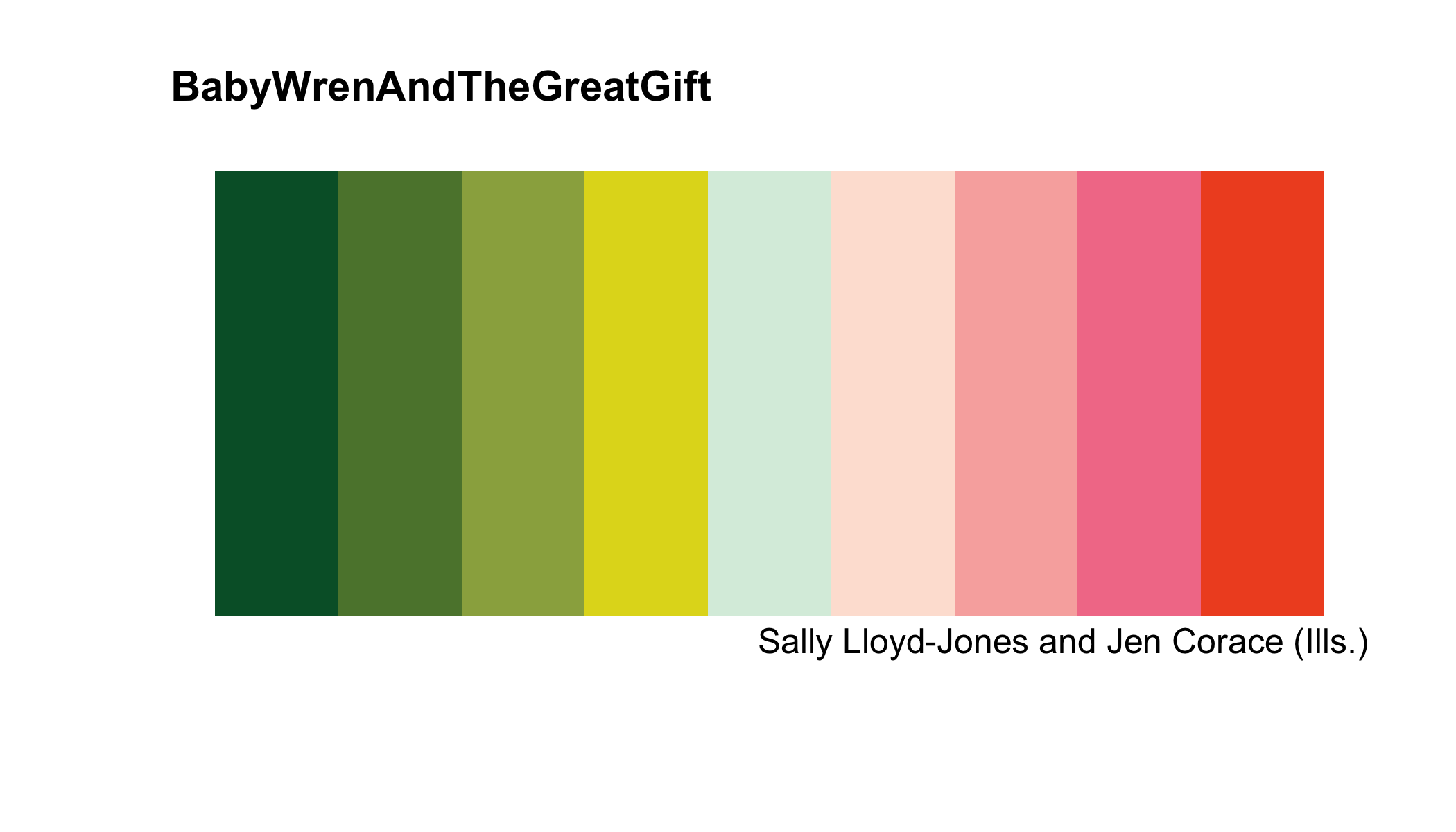
ShowBook()

Similar to ShowBookshelf() which shows all palettes with given filters, but ShowBook() is used to display a single book as a modified plot object.

ShowBook(name ="BabyWrenAndTheGreatGift")

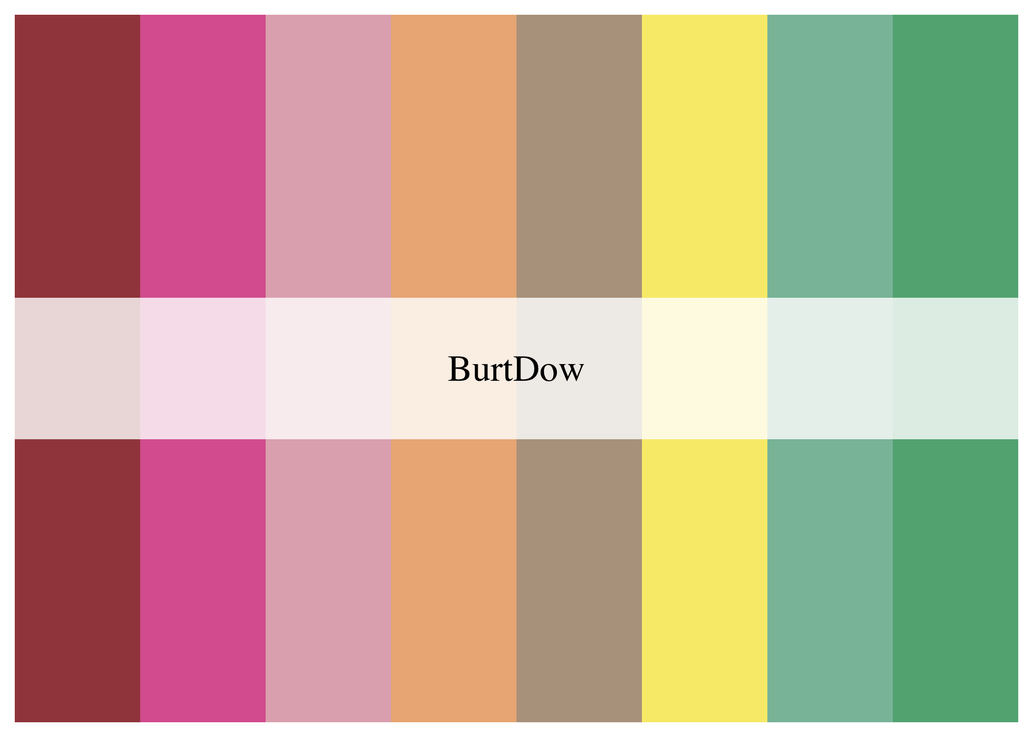
WB_brewer()

Select/create palettes from Wren’s bookshelf. Can create “discrete” or “continuous” color palettes using the type argument.

WB_brewer("BurtDow")

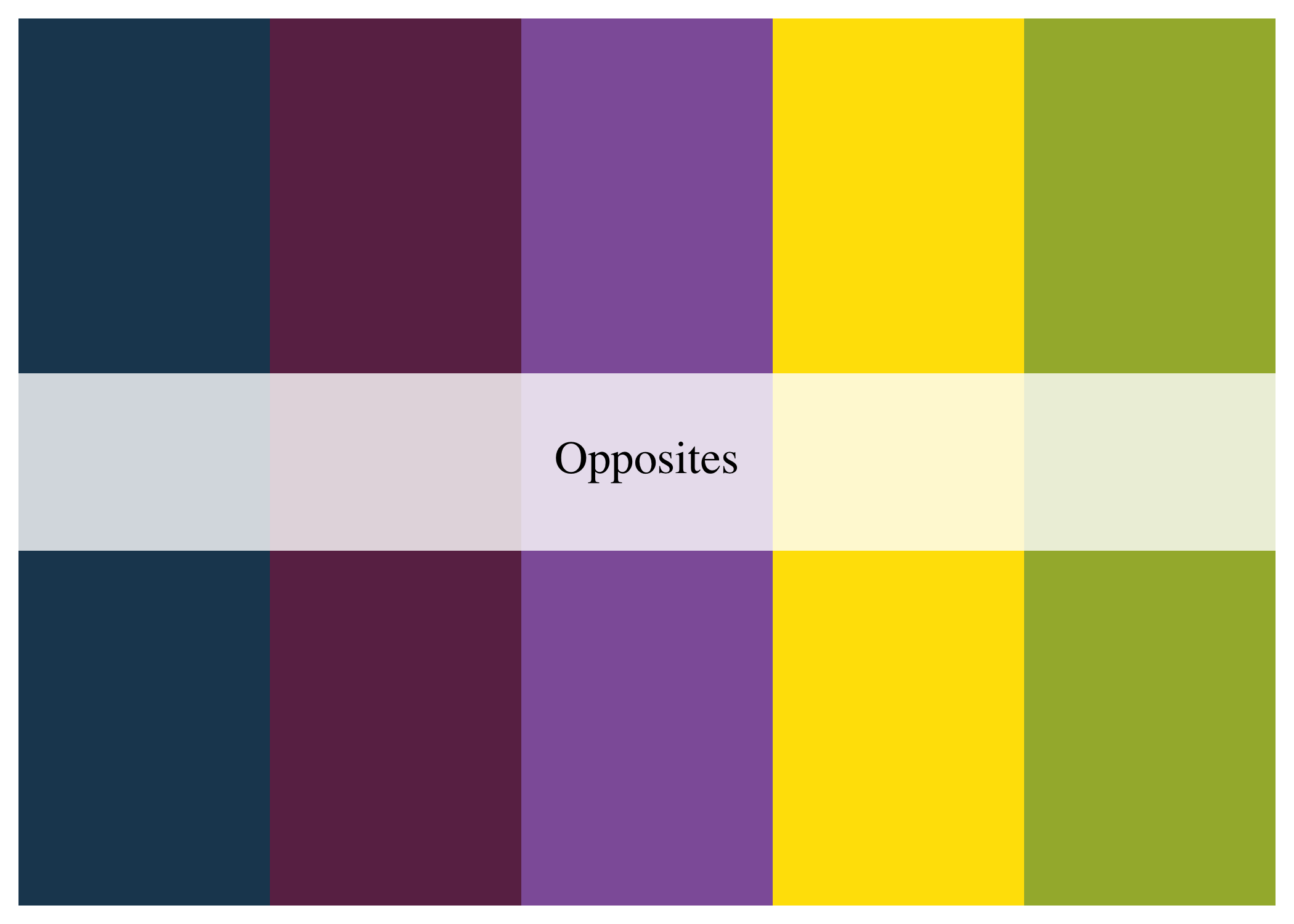
WB_brewer("Opposites", n = 5, type="discrete")

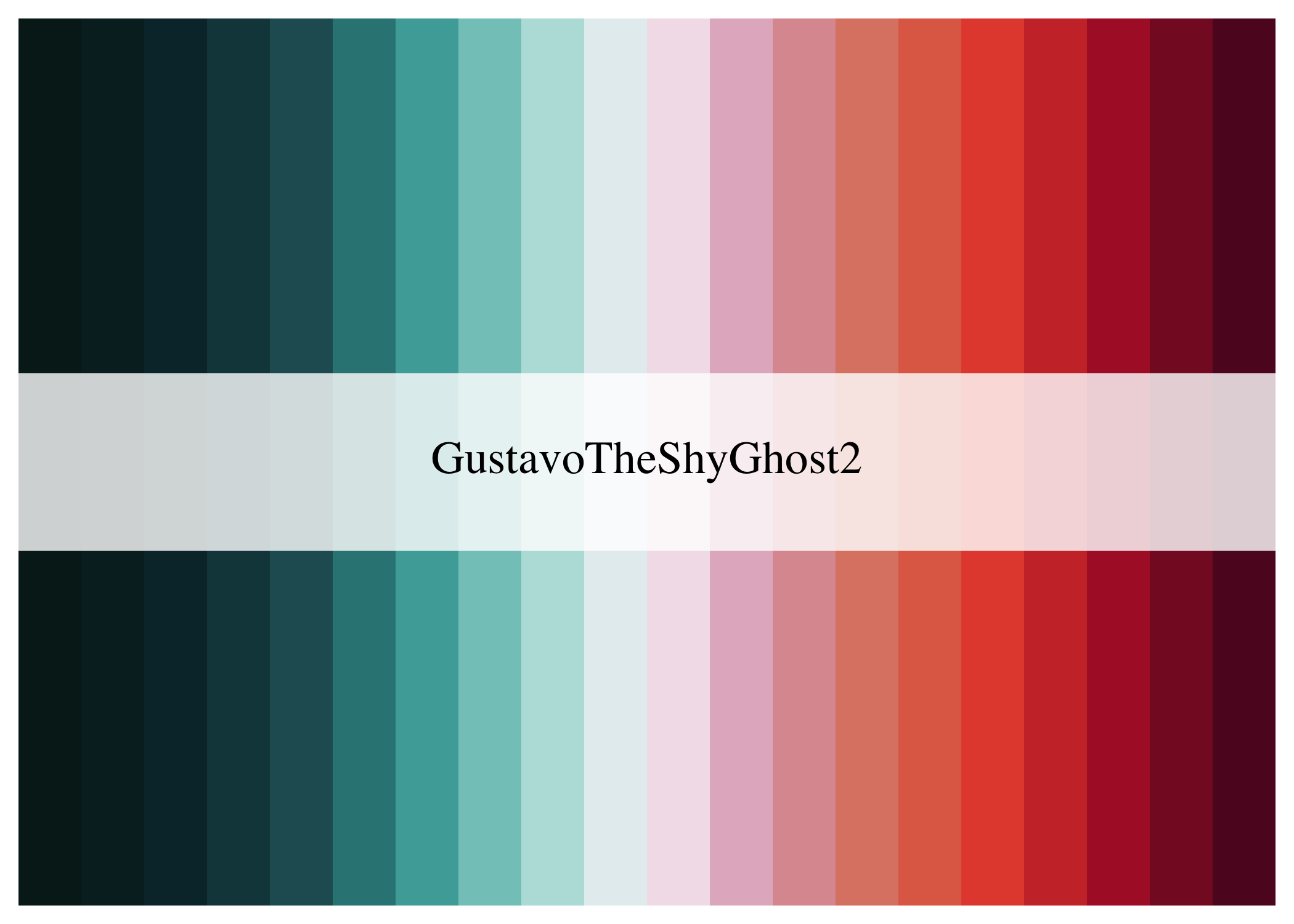
WB_brewer("GustavoTheShyGhost2", n = 20, type="continuous")

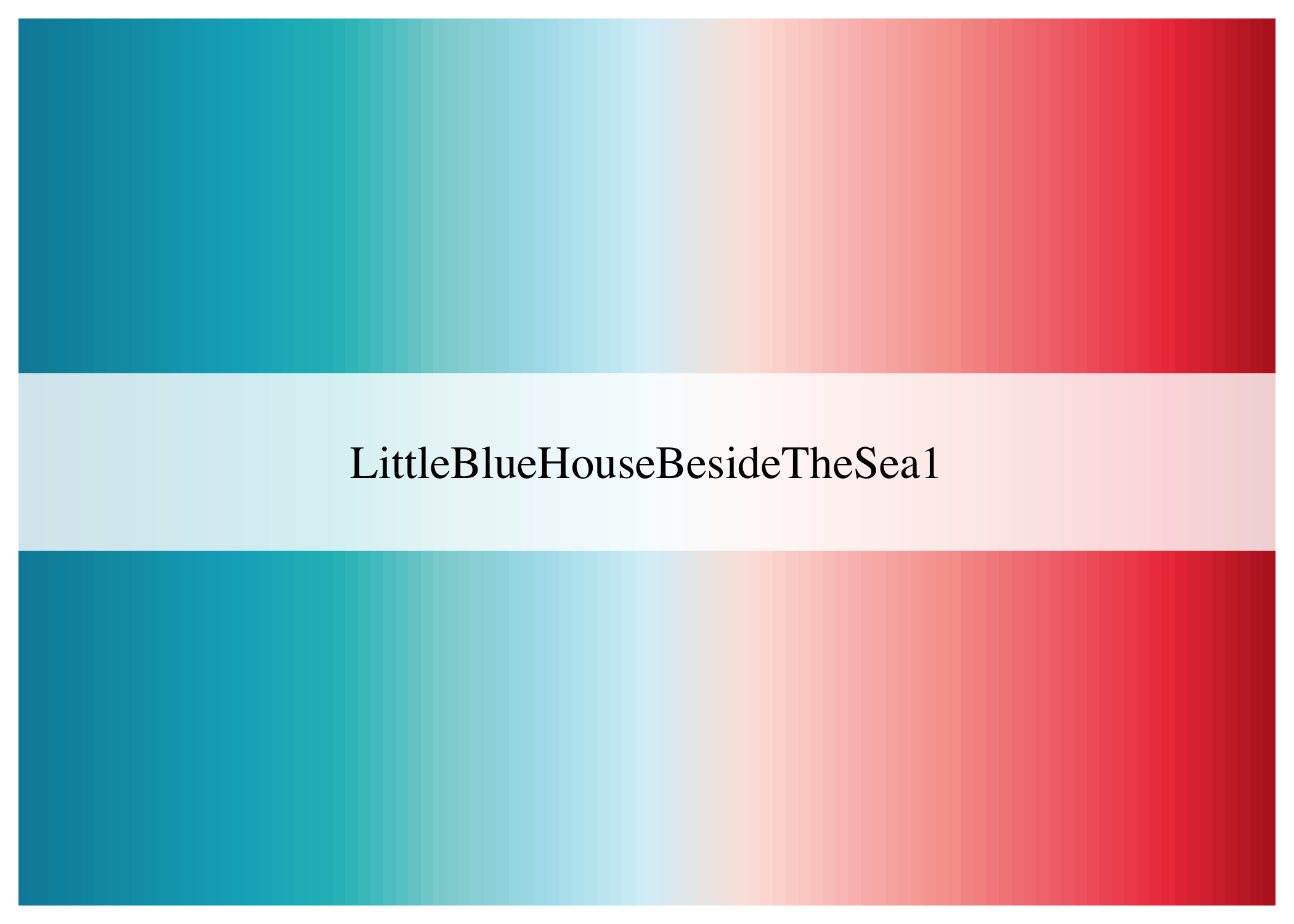
WB_brewer("LittleBlueHouseBesideTheSea1", n = 100, type="continuous")

For discrete palettes, I have assigned a specific order that the colors will be selected from a given palette when n < length(palette) in order to give the best contrast between discrete variables (in my opinion). This can be removed using override.order= TRUE.

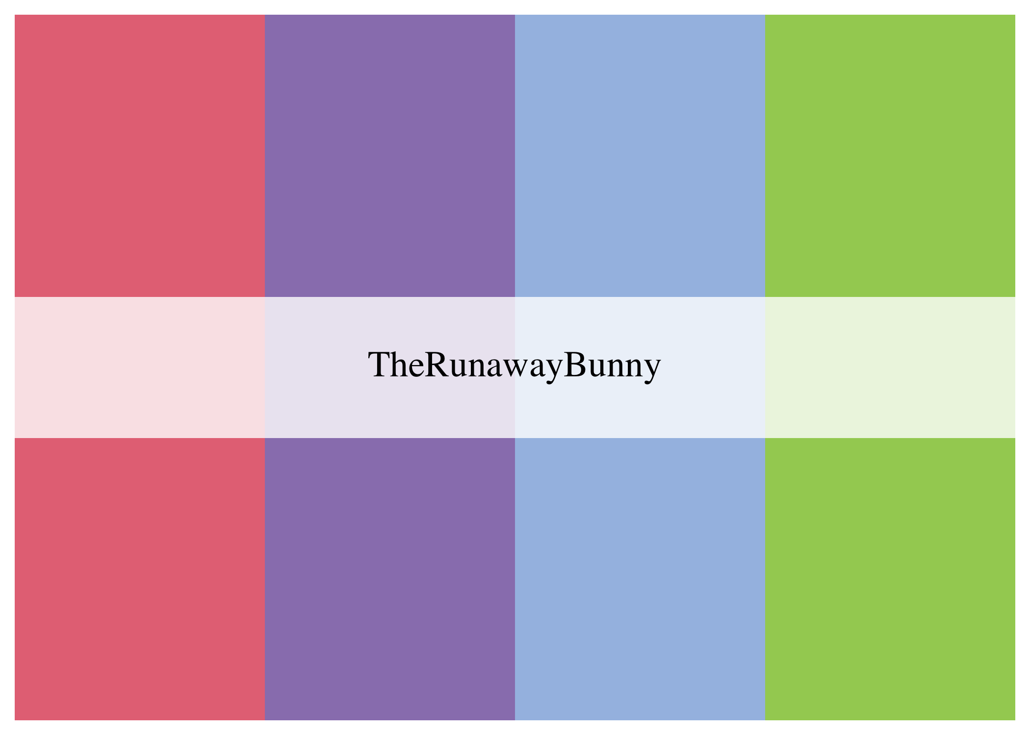
WB_brewer("TheRunawayBunny", n = 4, type = "discrete", override.order = FALSE)

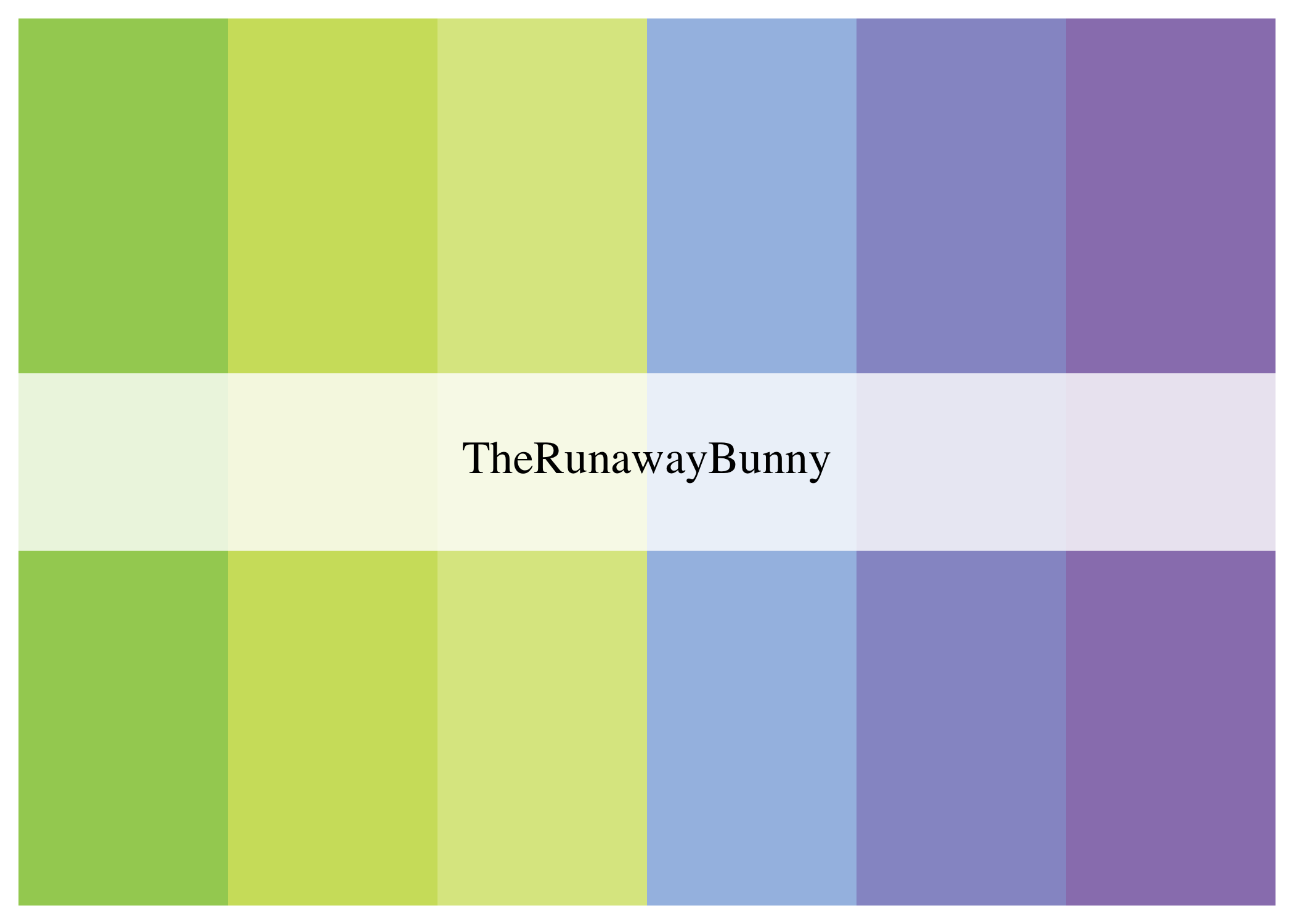
WB_brewer("TheRunawayBunny", n = 6, type = "discrete", direction = -1, override.order = TRUE)

WB_subset_brewer()

This function is just another way of customizing palettes that I tried building before figuring out a better way to do it. So, this is a relic that still works, and still gives a little more intuitive(to me at least…) or specific control over the final product.

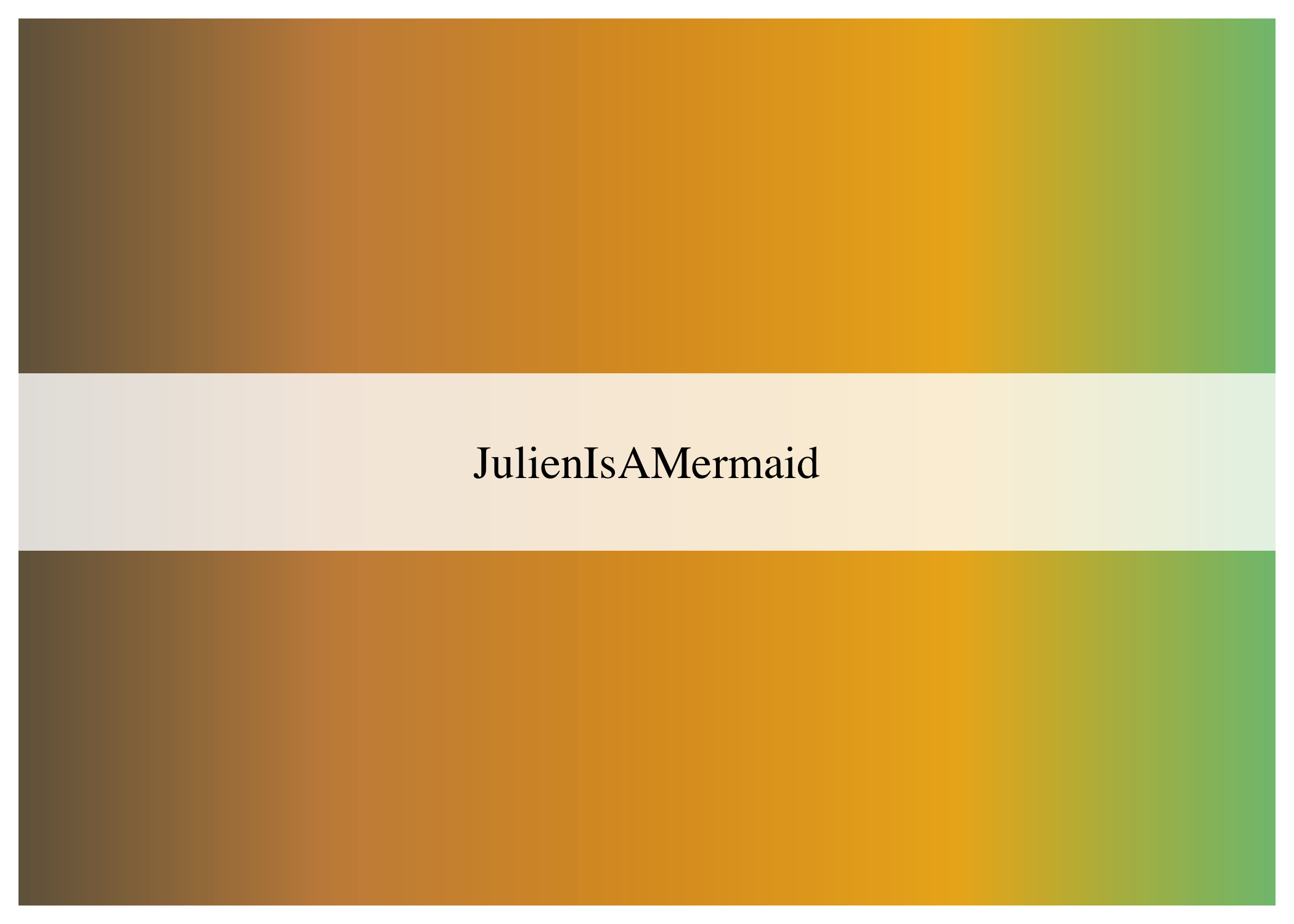
WB_subset_brewer(name = "JulienIsAMermaid", n = 5, LCR = "left", type = "continuous", n2 = 200)

It also allows for you to select the exact subset of colors you want from a palette by providing a vector of the colors positions (Left to Right) as shown by ShowBookshelf() or ShowBook() to the LCR argument. The vector you provide can also shuffle around the order of the colors to best suit your preferences.

WB_subset_brewer(name = "WhereTheWildThingsAre", type = "discrete", LCR = c(1,6,4,5))

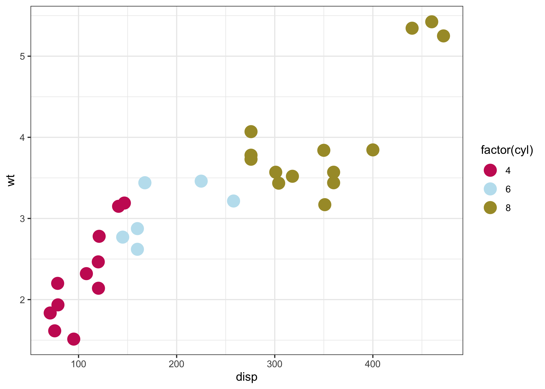
ggplot wrapper functions

Some convenience functions to make integration of palettes into ggplot2 easier.

library(ggplot2)
ggplot(mtcars, aes(x = disp, y = wt, color = factor(cyl)))+
  geom_point(size = 5)+
  scale_color_WB_d(name = "YouMatter")+
  theme_bw()

ggplot(mtcars, aes(x = disp,y = wt, fill= mpg))+
     geom_point(size=5, shape = 21)+
     scale_fill_WB_c(name = "ThisMooseBelongsToMe", direction = -1)+
     theme_bw()

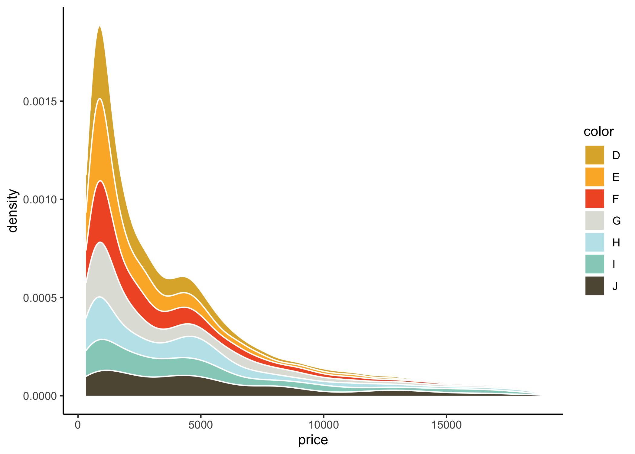
ggplot(diamonds, aes(x = price, fill = color))+
  geom_density(position="stack", color = "white")+
  scale_fill_WB_d("CapsForSale", override.order = TRUE)+
  theme_classic()

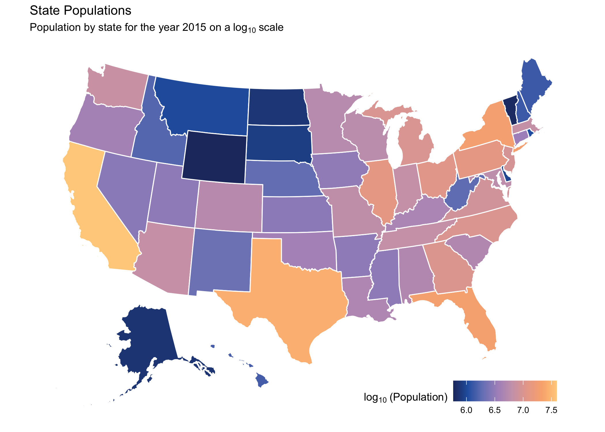
Can also simply utilize WB_brewer() within the normal ggplot2 scale functions.

library(usmap)
library(magrittr)
library(dplyr)
statepop2 <- statepop %>% 
  mutate(logPop = log(pop_2015, base = 10))
plot_usmap(data = statepop2, 
           values = "logPop",
           regions = "states", 
           color = "white") + 
  labs(title = "State Populations",
       subtitle = expression('Population by state for the year 2015 on a'~'log'[10]~'scale'),
       fill = expression('log'[10]~'(Population)')) + 
  scale_fill_gradientn(colors = WB_brewer("WhatWellBuild"))+
  theme(panel.background=element_blank(),
        legend.position = c(0.6,0.01),
        legend.direction = "horizontal")

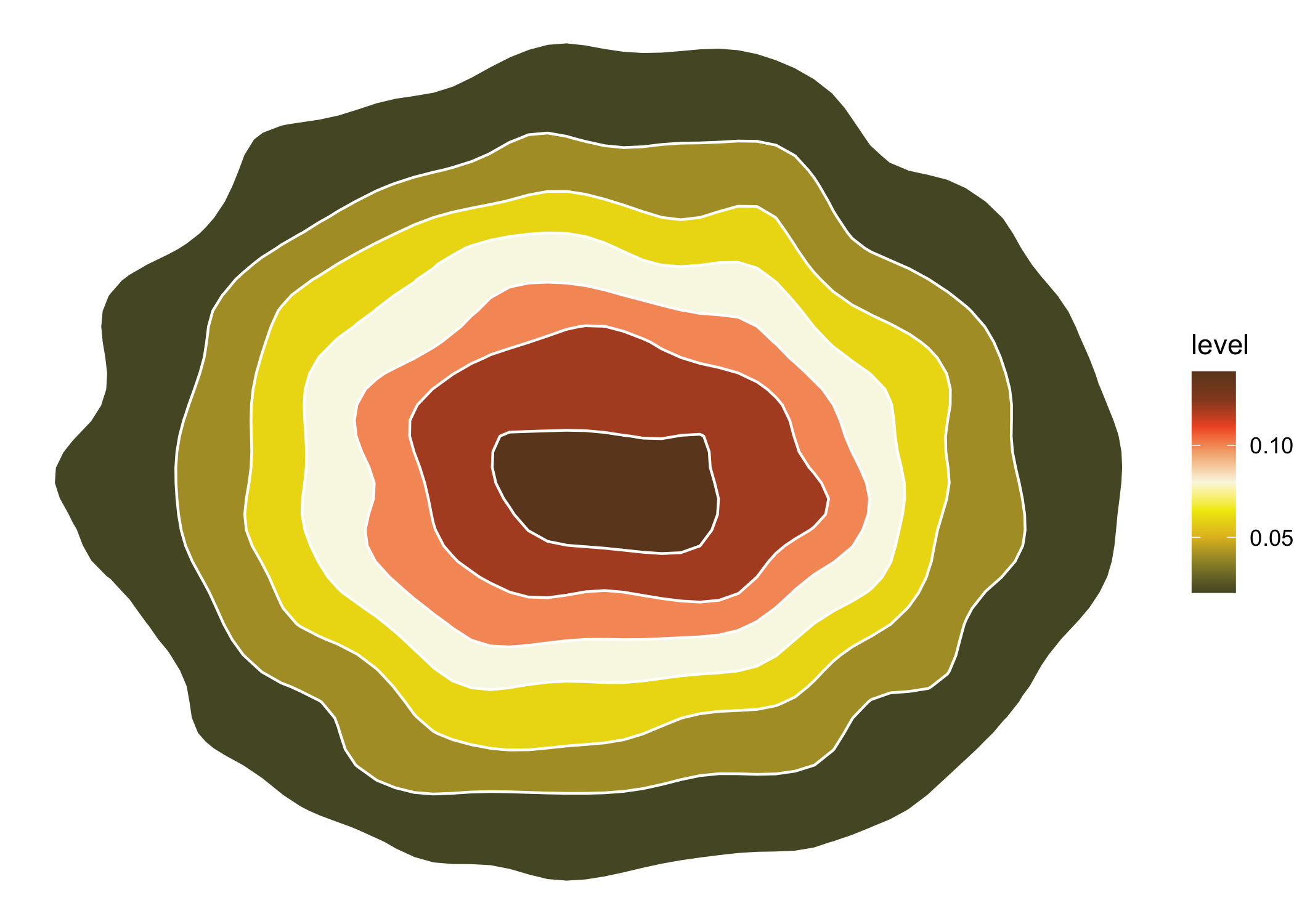
ggplot(data.frame(x = rnorm(10000), y = rnorm(10000)),aes(x=x,y=y))+
  stat_density_2d(aes(fill = ..level..), geom = "polygon", colour="white")+
  scale_fill_WB_c("TinyPerfectThings",direction = -1)+
  theme_void()